AGRICULTURE
High-precision localisation and navigation are at the centre of vital operations across diverse industries worldwide. These applications rely on highly accurate and reliable global navigation satellite system (GNSS) positioning. To achieve the level of precision required, several satellite and atmospheric errors must be resolved, typically through receiving GNSS corrections information, or by algorithms in the receiver.
One of the greatest sources of error is the refraction (bending) and diffraction (scattering) of GNSS signals by charged particles as they pass through the ionosphere (Table 1). To make matters worse, we are currently experiencing the upswing of Solar Cycle 25, resulting in increased ionospheric activity. The level of ionospheric activity depends on your location, time of day and time of year. After sunset in certain equatorial regions, you can almost set your watch to it!
| Contributing source | Error range |
|---|---|
| Satellite clocks | ±2 m (6.6 feet) |
| Orbit errors | ±2.5 m (8.2 feet) |
| Ionospheric delays | ±5 m (16.4 feet) |
| Tropospheric delays | ±0.5 m (1.6 feet) |
| Receiver noise | ±0.3 m (1 foot) |
| Multipath | ±1 m (3.3 feet) |
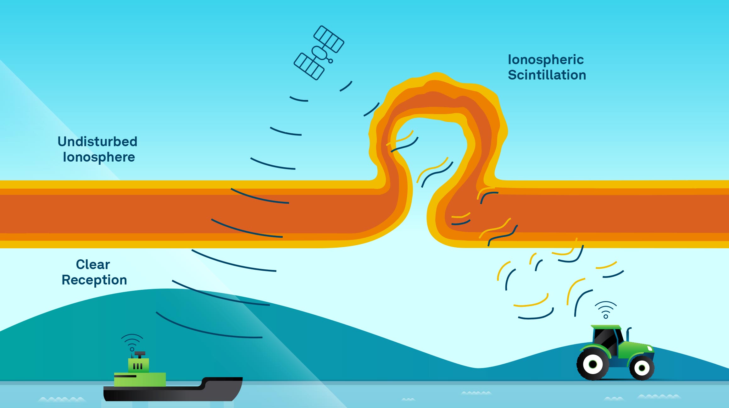
Further, ionospheric scintillation — rapid temporal fluctuations in GNSS signal strength and phase — is caused by small-scale irregularities in electron density called plasma bubbles (Figure 1). Because the time and location of scintillation are highly variable, it’s even more important to understand how the quality of your positioning may be affected to mitigate operational delays, safety risks and downtime.
This short article shows how you can use GNSS software to observe whether your positioning is being impacted by ionospheric scintillation or radio frequency (RF) interference, enabling you to make informed operational decisions.
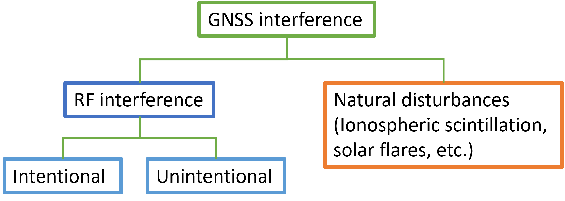
The United Nations Office for Outer Space Affairs (UNOOSA) International Committee on GNSS (ICG) classifies GNSS interference into two categories: RF interference and natural disturbances (Figure 2). While both can result in disruptions to GNSS positioning, how they affect GNSS signals differs, enabling users to distinguish what they are experiencing through software tools. Discerning what is affecting GNSS signals, which ultimately impacts positioning accuracy or even the ability to maintain positioning, is paramount to determining the best course of action.
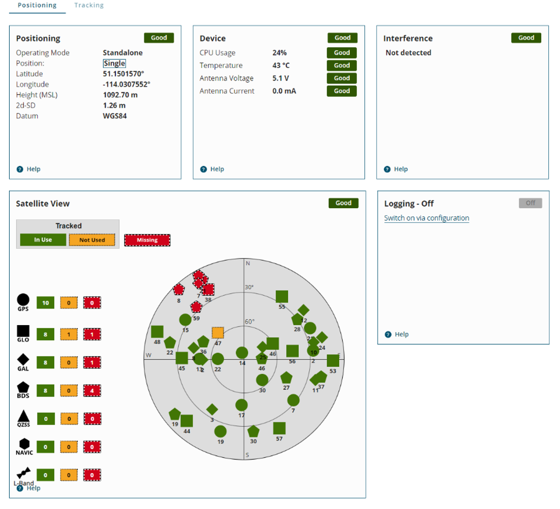
As an example, the NovAtel Application Suite provides an at-a-glance Positioning dashboard for your GNSS receiver status, including the tracked satellites by constellation and L-band corrections in the Satellite View box and RF interference detection in the Interference box (Figure 3).
High-precision GNSS receivers use advanced firmware algorithms to indicate the presence of RF interference. For example, OEM receivers by NovAtel have GNSS Resilience and Integrity Technology (GRIT) functionality including the Interference Toolkit (ITK) and Spoofing Detection (SD) modules to identify and detect RF interference. GRIT alerts the user enabling them to mitigate RF interference by applying digital filters. The NovAtel Application Suite dashboard has a simple indicator for RF interference detection by GRIT. If the indicator is Good (green), the receiver is not experiencing RF interference.
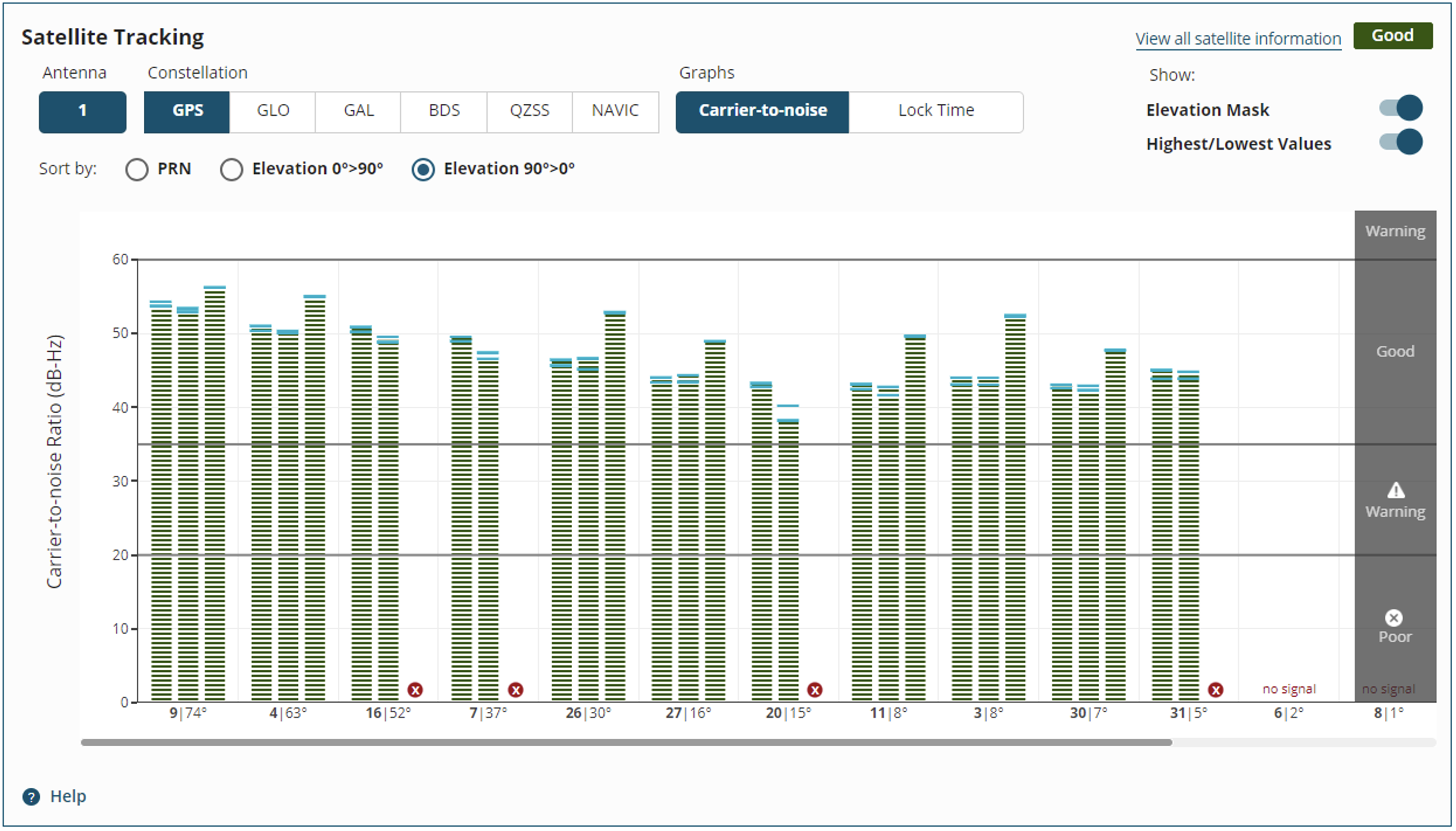
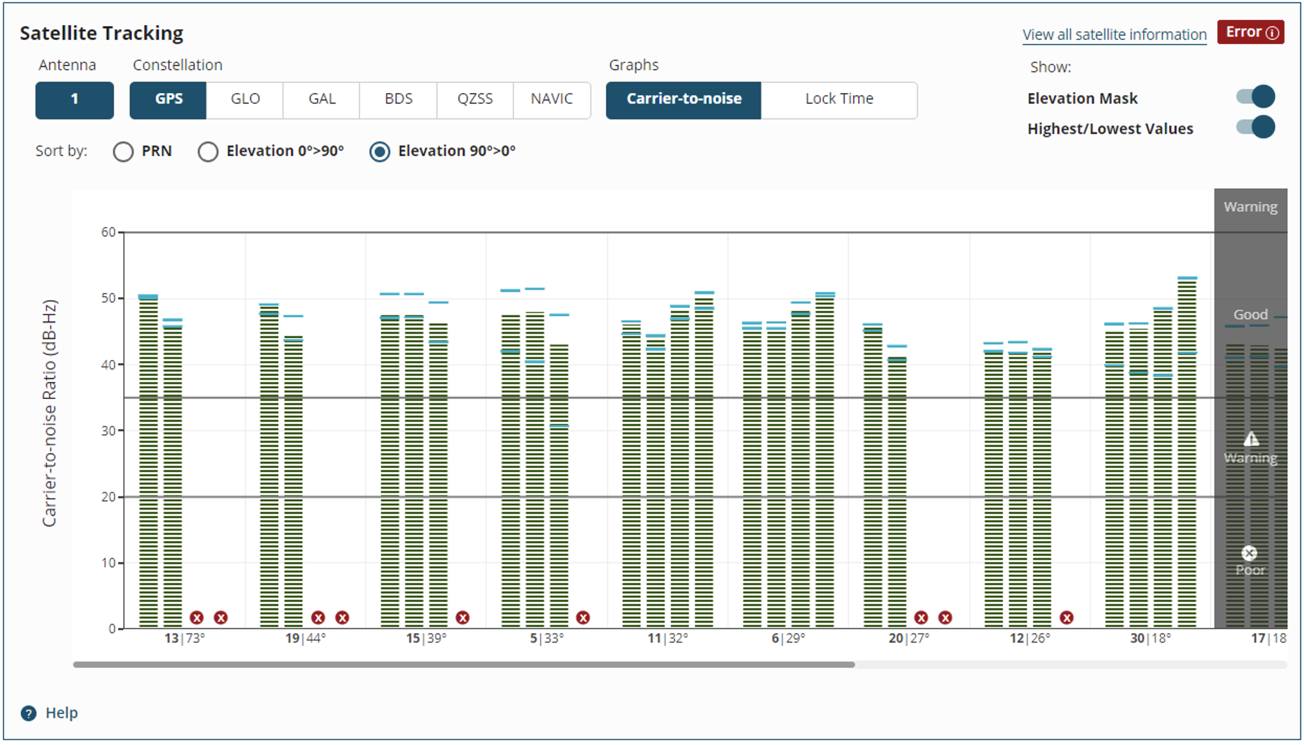
From the Positioning dashboard, you can toggle to the Tracking dashboard to view the carrier-to-noise ratio (C/N0) and lock time graphs by constellation (Figure 4 & 5). In both cases, for each satellite indicated on the x-axis, the vertical bars represent individual GNSS frequencies (e.g., L1, L2, etc.) transmitted by that satellite. In this way, you can see how multiple frequencies are behaving in a single view. This view also allows the user to toggle through the different GNSS constellations.
As mentioned, ionospheric scintillation presents as a rapid, temporal fluctuation in GNSS signal strength (C/N0) and phase across all GNSS frequencies. We emphasise the latter because it is a distinguishing factor compared to RF interference, which is typically observed in one or two bands.
For example, the graphs in Figure 4 show the C/N0 for satellites in the GPS constellation under normal conditions (panel A) and with high signal variation (panel B) indicated by the separation between the upper and lower blue bars. In these graphs, the green column shows the signal strength in real-time, and the blue bars are the highest and lowest measured values updated every second. What is key to note in Figure 4B is that the high signal variation is seen across multiple frequencies. In addition, more frequencies are not tracked (red circles with X) than under normal conditions.
The red error flag in the top right corner serves as a quick indicator of an anomaly for overall tracking health. The user can click on the flag to learn what the error is, which in this example is due to the high signal variation.
A
B
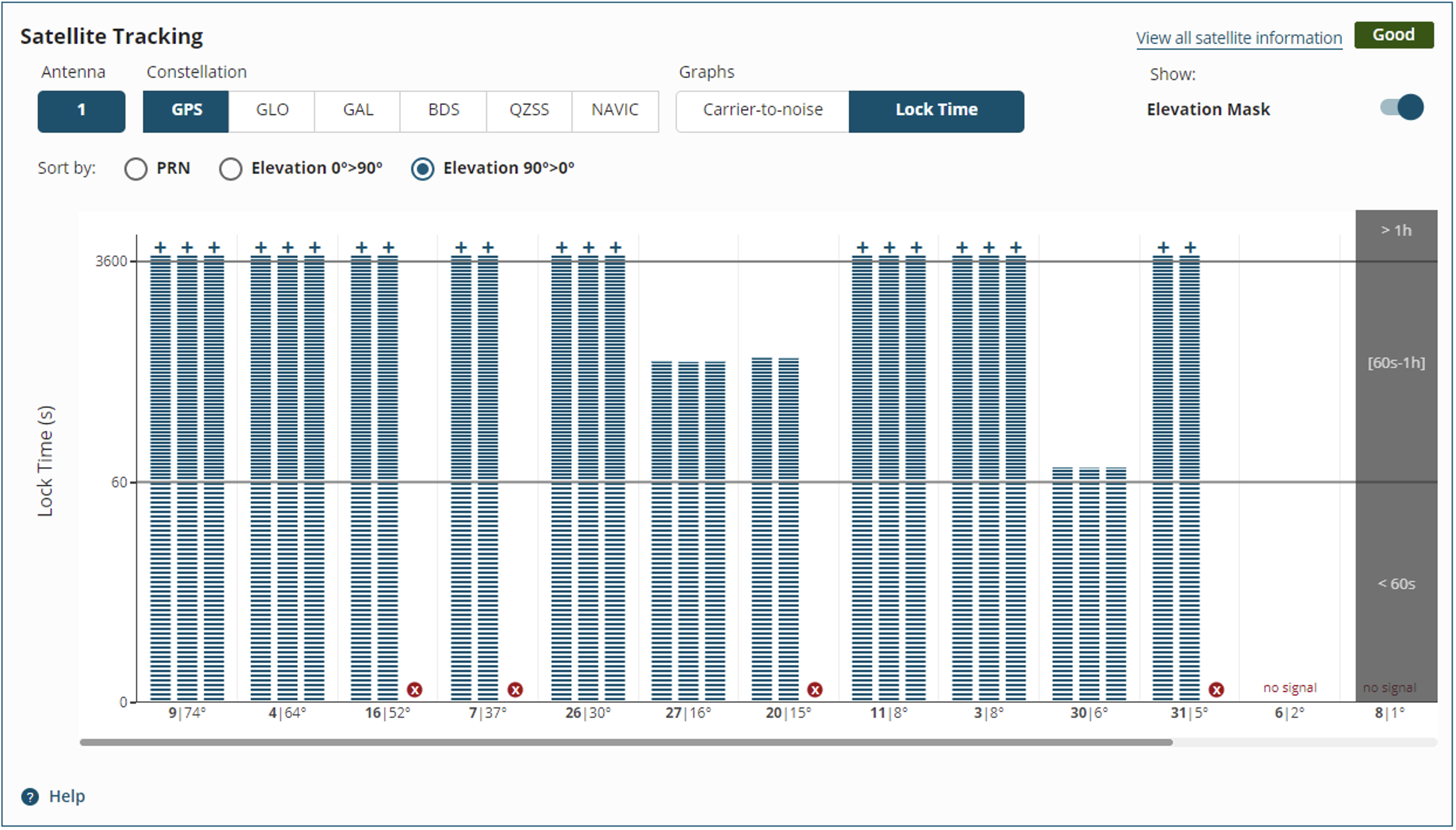
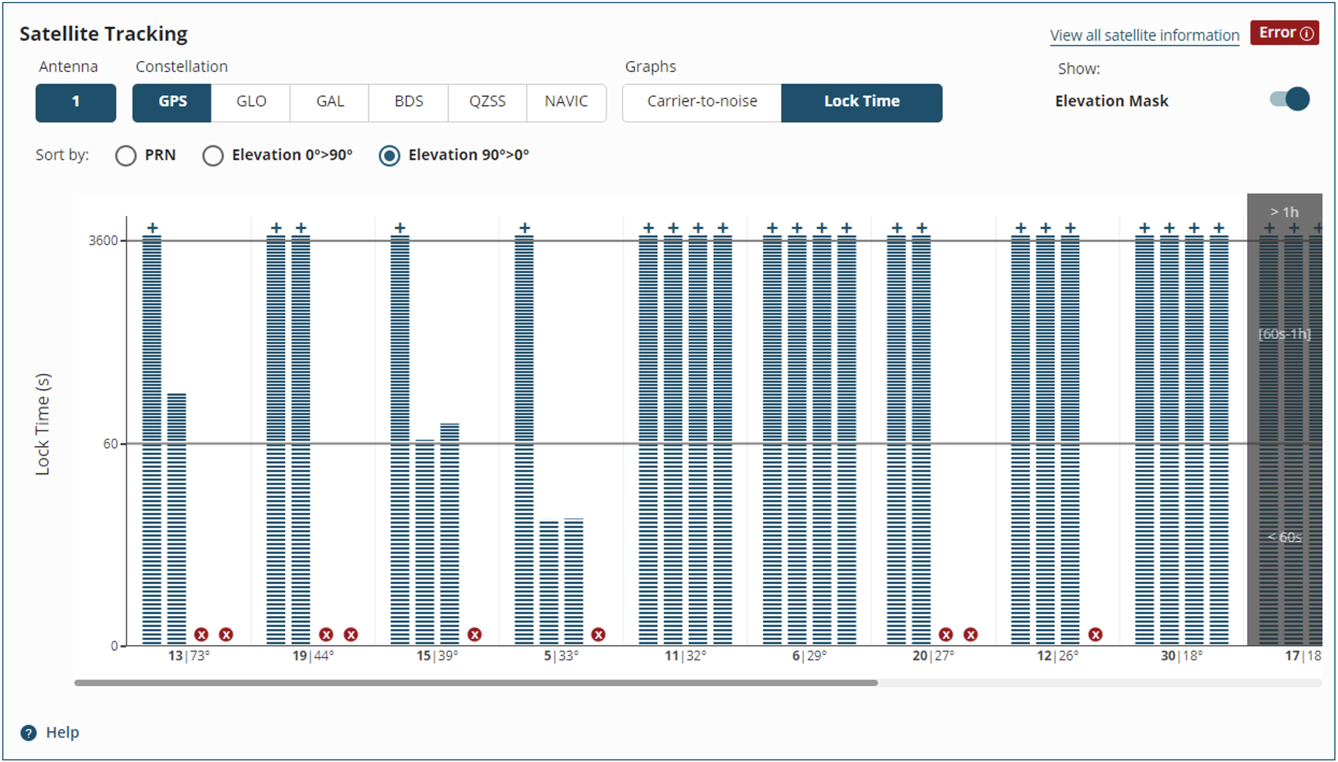
Lock time is also adversely affected by ionospheric scintillation as the length of time signals are continuously tracked decreases (Figure 5). The presence of scintillation is reflected by shorter lock times (more bars at or below 60 sec) as well as loss of lock (red circles with X) than under normal conditions.
A
B
To corroborate whether the data shown indicates ionospheric scintillation, you can refer to an ionospheric activity forecasting tool that monitors the regional and temporal changes in total electron count (TEC). If the timing and location where you experienced GNSS signal anomalies coincide with high ionospheric activity, any positioning issues experienced are very likely due to scintillation.
As with any interpretation of raw measurements, there is always a chance of false positives and false negatives. In this case, a false positive would conclude that the observed effect on GNSS positioning was due to scintillation, when it was due to other factors. A false negative would conclude that the observed effect on GNSS positioning was not due to scintillation when it was.
For example, cabling issues can cause the strength of all frequencies to be consistently low versus the fluctuation seen with scintillation. Installation problems such as placing the antenna too close to other electronic devices can cause abnormalities in the received GNSS signals. As discussed, RF interference also typically affects one or two discrete frequencies rather than all signals.
While you cannot completely avoid the possibility of false positive and negative scenarios, observing rapid fluctuations in signal strength for all GNSS constellations and frequencies while your receiver is in a region experiencing high ionospheric activity is a strong indicator of scintillation, particularly when the software does not detect RF interference.
Ultimately, whether you need to be concerned about ionospheric scintillation or not is if your operations are affected by any reduction in GNSS positioning solution accuracy or availability. Having software visualisation and forecasting tools at your disposal can help narrow down if ionospheric scintillation is the issue and guide next steps.
To learn more about ionospheric activity and scintillation, check out our other resources and sign up for updates.
If you need assistance with ionospheric scintillation, please contact us for support.